In the late 80s Udo Pachner introduced the idea of a bistellar move which can modify the triangulation of an object (simplicial manifold) without changing its fundamental properties (topological type). About a decade later, Frank Lutz implemented bistellar_simplification as a tool to classify objects by their topological type using a simulated annealing strategy. Later, Niko Witte wrote a C++ implementation of Frank’s code for polymake, which considerably sped up the computation. I, then, spent several (loong) months trying to improve Niko’s code so that it can be used to recognize our spheres.
The 2-dimensional version of a bistellar move is well known in the graphics community, though it is usually called by a different name: edge flips. It can be used to find “nice” triangle meshes of some domain, which may, for example, be applied to finite element-type computations.
The idea of the bistellar move is simple. We’ll be using some terminology from here. Let’s start with a simplicial complex [latex]K[/latex] of dimension [latex]d[/latex] and a simplex [latex]\sigma \in K[/latex] of dimension [latex]0\le i \le d[/latex]. (Technically, [latex]K[/latex] should be a closed combinatorial manifold.)
A bistellar [latex]i[/latex]-move is [latex]\Phi_K(\sigma) = K – \text{star}(\sigma,K) + \tau \ast \partial \sigma[/latex], where [latex]\tau[/latex] is a [latex](d-i)[/latex]-simplex NOT in [latex]K[/latex] such that [latex]\partial \tau = \text{link}(\sigma,K)[/latex]. The move is only valid if a [latex]\tau[/latex] satisfying these properties exists.
The animated gif below shows some bistellar moves in action. You can see why the algorithm is called a bistellar simplification — we can change the triangle mesh to have fewer triangles.
Consider an abstract graph whose nodes are simplicial complexes which are connected by an edge if there exists a single bistellar move to get from one complex to the other. This graph is known as the bistellar flip graph or Pachner graph. The bistellar_simplification algorithm is equivalent to a random walk on this infinite graph which attempts to identify the topological type of the input complex [latex]K[/latex] by lowering the [latex]f[/latex]-vector of [latex]K[/latex].
Tracking the [latex]f[/latex]-vector is the cheapest way to track our progress of the simplification. In fact, for a 4-dimensional sphere, the number of vertices and edges alone is enough to learn about the entire [latex]f[/latex]-vector [Klee]. So we can actually track the progress of the simplification on a 2 dimensional graph.
Below is a video tracking the progress of our modified bistellar_simplification on our Akbulut-Kirby 4-sphere AK_I_3. Since following a single dot was difficult to see, I am displaying the [latex]f[/latex]-vector (or, more precisely, just the vertex and edge count) of 1000 consecutive complexes at a time. For each of those 1000 complexes, I counted the number of 0-,1-,2-,3-,4-dimensional bistellar moves were made (red = 4-move grows the [latex]f[/latex]-vector, green = 0-move makes [latex]f[/latex]-vector smaller; green = good). The box on the bottom right displays the vertex and edge count of the complex at the specified round.
Notice that the simulated annealing strategy brings the [latex]f[/latex]-vector down until it gets stuck for a while, then it grows the [latex]f[/latex]-vector in an attempt to jiggle the complex out of the local min. The current implementation uses a greedy random strategy, the modifications we made to the strategy only improved the algorithm enough to recognize AK_I_3, AK_II_3, AK_III_3. The other spheres to our knowledge have not been recognized by any heuristic software we know of.
We have also tried to implement a Markov chain Monte Carlo (Metropolis) method to improve the algorithm. We have tried several different parameters for the energy. Our tests so far indicate that an MCMC strategy results in a significant slow down of the algorithm. We are now looking into testing other deep learning techniques.
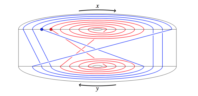 We then want to glue two 4-balls onto this manifold to close up the two holes that we introduced when we attached the two one-handles in the beginning. But we will glue them on in a non-trivial way. We will follow along the two paths (red and blue) shown above. If you start from the blue dot and walk along, you’ll find the blue path goes along the [latex]x[/latex]-handle, then [latex]y[/latex], then [latex]x[/latex], then the [latex]y[/latex]-handle backwards, then [latex]x[/latex] backwards, then [latex]y[/latex] backwards, and return to the blue dot. We describe this blue path as [latex]xyxy^{-1}x^{-1}y^{-1}[/latex] and the red one is [latex]x^5y^{-4}[/latex].