During this strange time, many organizations have opened up their media to the world. I’ve collected the ones I learned about from my wonderful community of social media friends and colleagues. I’m just copy-pasting from them without credit, and in no particular order. This is not at all my hard work, it’s theirs. So thank you, friends!
Note: Some of these are free only for now. Some are free for a trial period with sign up. Some come with a small fee. Some are always free.
Khan Academy – Especially good for maths and computing for all ages but other subjects at Secondary level. Note this uses the U.S. grade system but it’s mostly common material.
BBC Learning – This site is old and no longer updated and yet there’s so much still available, from language learning to BBC Bitesize for revision. No TV licence required except for content on BBC iPlayer.
Futurelearn – Free to access 100s of courses, only pay to upgrade if you need a certificate in your name (own account from age 14+ but younger learners can use a parent account).
Seneca – For those revising at GCSE or A level. Tons of free revision content. Paid access to higher level material.
Openlearn – Free taster courses aimed at those considering Open University but everyone can access it. Adult level, but some e.g. nature and environment courses could well be of interest to young people.
Blockly – Learn computer programming skills – fun and free.
Almost every week for the last 2 years, I’ve been teaching in a live virtual classroom. Here are some things I’ve learned.
Test your equipment ahead of time
Obviously you’ve already tested the software and hardware to see if you can use it all and where the buttons are. That’s not what I mean. I’m saying that you should really know what it’s like to be on camera, to see yourself on camera while you’re speaking. It’s not at all like speaking in an in-person classroom.
You may feel self-conscious if you don’t often see yourself talk. It’s like when you see a video of yourself. (I don’t sound like that, do I?) It’ll feel awkward in the beginning, like you’re talking to yourself. You might notice yourself saying something or doing something repeatedly, which might make you to feel more stressed, which could cause you to do that thing even more, which’ll make you more stressed, and …. If you feel yourself going there, you have to take a breath and calm down. Slow your speech. Take a break.
You may not be able to see your students’ faces or their reaction to what you’re saying. Even when you ask them to react in the chat most of them likely will not. You don’t know if you’re talking to yourself or to students who are really paying attention but too shy to type anything in the chat. This is very different from an in-person classroom where non-verbal communication speaks volumes.
Try getting a reaction from students relatively frequently. “Give me a plus if that makes sense and you’re ready to move on. Give me a minus if you want me to explain it again.” Don’t give them the third option of abstention. It won’t be a substitute to seeing their eyes light up, but it might help a bit.
Have a “going to work” ritual
Even if you’re teaching from home, get showered and dressed as you would if you were going to campus. Go get a coffee, if that’s something you used to do every day. You need to psych yourself up before teaching. You may not think you need to do this, but it’ll make a difference in your level of concentration. You need to create some artificial signal so you can leave your “home stuff” at the door and get into prof mode before going on screen.
Take frequent breaks and move around
Ever see a student pass out while you’re teaching? It’s annoying because they fell asleep while you were looking right at them. Well, with nobody looking at them, it’s a lot easier for them to drift off to dreamland or get distracted. Virtual classes require more mental breaks than in-person classes. You’ll need to work that into your teaching.
And when you take those breaks, YOU (and the students too) should get up and stretch, walk around. Don’t just sit through the break even if you have some emails to check. They can wait. You’re used to teaching while standing at a podium or walking around. Your physical body exerts energy to be able to do that, blood is rushing and moving oxygen. It will make a difference in the way you speak and think.
Make time to chat with your colleagues
If you’re used to making small talk with the administrative staff or catching up with friends in the mail room, you’re more social that you may give yourself credit for. And it’s going to be important to continue to maintain some of that social life to keep yourself happy. You may not feel it in the first 2 or 3 weeks. But sooner than later, you may find your anxiety levels increase, your ability to focus decrease, or other mild symptoms of depression start to appear. Schedule online tea time with some of your colleagues at least once a week so you can meet your social quota for the week.
Don’t forget we’re ALL going through this
And finally, as difficult as it is for you to get through this transition, it’s no cake walk for your students either. They need to keep their sanity as well. READ THIS BLOG and remember that we’re all under a lot of stress right now.
Also, you may think that being extra flexible is showing kindness or understanding to your students. It may not work out that way for some students. In this confusing time, I suggest that you not give them more options, more uncertainty. Set well-defined boundaries so that at least this part of their life has stability. Any student who cannot fulfill any part of your requirements will come to you in private, as usual, and you may show mercy to them then on a case-by-case basis.
There are many sources being shared for how to deliver an online course. Read them, learn from them. Here, I want to emphasize that it’s important to take care of yourself, too, now. There are others who will surely benefit from your guidance.
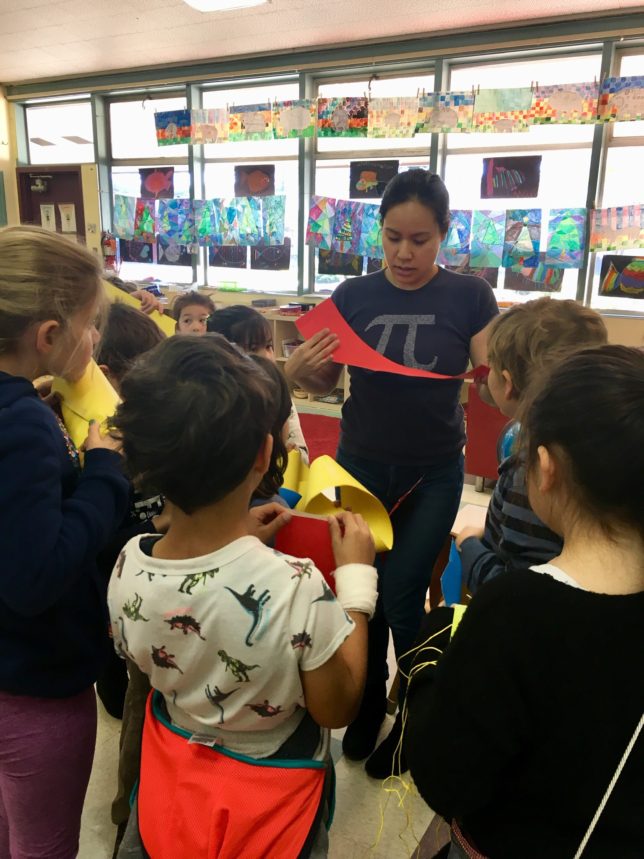
This year for Pi Day, I decided to go to my daughter’s 1st grade class to talk to the kids about math. After posting the above photo in my social media account, I got a few questions about what I taught. I figured I might as well write it down for preservation since I did spend some time thinking about it and felt it went quite well. Also, this way I can refer back to this blog later, when the younger one is in 1st grade 🙂
I need to begin with a few notes. My daughter attends a private school. Why does this matter? For one thing, the class size is small. This 1st grade class has 17 children, all of whom recognize and are comfortable around me.
Also, the school’s teaching style is not at all what I experienced in public school in Queens, NY (back in my day…). The teachers provide a unique learning program for each student matching the student’s individual learning style.
Putting those things together, we have a group of students who are not afraid to try new things, even with someone they’re not used to learning from. The following lesson plan happened to work in my daughter’s class, but I don’t know if it would work in a larger class, for example. Anyway, let’s get started.
Introduction
I introduced myself as a mathematician. My daughter’s class is full of girls. Of the 17 students, only 5 are boys. So it was important to me to tell the girls that I am not just someone who likes math. I am Fr. Dr. Mimi. I spent more years in school after high school than before it. I spent 15 years studying mathematics! And now that I studied so much more math than most people in the world, it’s my responsibility to teach math to anybody who wants to learn about math from me.
And today, I want to talk to you all about math because today is a very special math day. Today is Pi Day! This letter on my T-shirt is a symbol that represents a very special number. You all spent a lot of time this year learning about counting numbers. This is a special number that isn’t a counting number.
This letter [latex]\pi[/latex] is actually a letter from the Greek alphabet. You all know what an alphabet is, right? A, B, C, D, … Some languages have different letters in their alphabet. In German there’s an ö and ü and ä. In Spanish there are letters that are different, like ñ. And in Greek there are also a bunch of letters like A.
What letter do you think “A” is? This is the letter alpha. This is the capital letter alpha. Here’s the lowercase letter alpha: [latex]\alpha[/latex]. Here’s capital and lowercase beta: B [latex]\beta[/latex]. And the next letter in the Greek alphabet is gamma: [latex]\Gamma \; \gamma[/latex]. And this is the letter pi: [latex]\pi[/latex].
The Greeks also have symbols for numbers. This is the symbol for one: I. And this is the symbol for two: II. Here’s the symbol for five: V. It actually doesn’t matter what symbol we use for numbers, as long as we all agree to use it. Numbers aren’t real. You can see or touch numbers the way you can see or touch a cat. Zero is a number that represents nothingness. And three is a number that represents how many things you have, but not the actual thing. Numbers are just ideas. Some numbers can be used for counting. But not all numbers are for counting. Pi is not a counting number. Pi is a very special number that has something to do with circles. And we’ll talk more about that later.
So far you might think that math is all about numbers. But that’s only because you just started learning math. When you start to read, you start with the alphabet, but eventually you start to form words using those letters. And then you combine words together using special rules to make sentences. And you combine sentences together to write stories.
Numbers are just like the alphabet. So 1 and 5 and 200 are all letters. Right now you’re learning about plus and minus. Well, 1+5=6 is a sentence in mathematics. And I’m going to show you today that you can tell stories in mathematics without using any numbers at all!
Distance
I am a very special kind of mathematician. I am a geometer. I study geometry. I don’t study numbers. I study shapes. So I’m going to talk to you all today about one of my favorite shapes. The circle.
Before we begin we have to start with a special word we use in mathematics: distance. Distance is used when talking about something far away. Distance is expressing exactly *how* far away that something far away is. Sometimes you might hear someone talk about short distances using a different word. Length. How long something is.
Now take a look at these two lines. Can someone tell me whether the length of these two lines are the same or different? What’s your guess?
A guess is also called a hypothesis. And that’s great place to start. Now I want you to show me that your guess is correct. How can you show me whether these two lines are the same or different?
I gave the kids a chance to play around drawing other lines on the board and drawing more lines with the giant triangle I used to draw the lines. Then someone suggested marking the giant triangle.
Great idea! You want to compare one line with the triangle and then compare the other line with the same triangle? I’ve actually brought some tools with me that you might be able to use to do exactly that.
I brought with me a bunch of rolls of colorful string. (Hemp string about 10+m each in 6 colors. Was on clearance at Target for $2.50. Cut them to be about 4m per student.) I used the string and measured out the length of one line, remembered it, and then brought it over to the other line to compare. I handed out a string to each student.
So these two lines are the same length! Is everybody here convinced? Does anybody still think that these two lines are different?
Geometry
Next I pulled out some colored paper. (I bought 3 giant poster-sized paper, also at Target, at about $0.69 each. They were not soft like construction paper, but rather stiff. I cut them to be about 4″x18″.) I handed one out to each student.
Now do you think these two (pink) edges of this paper are the same or different. Show me!
Now tell me if these two edges are the same or different. Show me! And see if you can find a way to show me without using the string. (Solution: Just bend the paper over to put the two edges together.)
Now we’re going to do something much harder. I got the paper and got some tape and taped the two short edges of the paper together to form a cylinder. I showed the two circles that form on the boundary of the cylinder. And I asked are these two circles the same length or different? What does it mean to ask about the length of something that’s curved?
To measure the circumference of the circles on the cylinder, I showed them that we could just use more tape and go around the circle using the string again. Because the string bends just like the paper bends. Once we get back to where we started taping the string down, we could probably cut the string. Then reuse that string to compare the circumference of the other circle.
But actually, I told them, we already knew that the two circles are the same. How?? Just open up the cylinder again and we get back the original rectangle! We can prove that the circles are the same “length” by reusing an older proof about the length of two edges of a rectangle. We never changed how long the edges are, so the lengths should still be the same even if it’s curved!
At this point, I think it would have been a good idea to spend a bit of time letting the kids play with this idea of the “length” of a circle. I feel now that I didn’t give them enough time here. I think it would have been better to let kids come up with their own ideas. For example, a diameter would be a perfectly reasonable attempt to measure the length of a circle. It’s unfair to assume that a circumference is the only length of a circle. And it would have been a great way to segue back to the conversation about [latex]\pi[/latex].
But I got ahead of myself and way too excited about the next thing I wanted to show them: a Möbius strip.
Once the cylinder was back to rectangle again, I showed them that we can just introduce a half twist to obtain what is called a Möbius strip. (I had to do the actual construction myself for every student.) I then asked them whether the circles on the edges of the Möbius strip are the same or different.
A bunch of kids immediately said they must be the same for the same reason as before. I think they had had enough by this point and few had the patience or attention span to complete this final task. But about 2 or 3 kids were still intrigued. They tried the trick of using tape to go around the edge and realized there’s only one circle. This seemed to surprise them, but not amaze them, which is the reaction I was hoping for.
Conclusion
At the very end, I spent about two or three minutes demonstrating to them what [latex]\pi[/latex] is. I got a string and measured the diameter of a circle and cut it. Then I cut another string for the circumference of a circle. And then show them that I need to get a little bit more than 3 of the short strings to get the long string. I explained that it doesn’t matter how big or small the circle is. You’ll always need a little bit more than 3 of the short ones to get the long one. And that number keeps showing up so many times in nature that we decided to give that number a special symbol [latex]\pi[/latex].
I’m pretty sure nobody got the message about [latex]\pi[/latex]. But my goal to begin with was to show the students that math does not have to be about numbers. Hopefully that message got through.
This lesson ended up taking just over an hour. I planned only to spend about 40 mins because I felt that’s the absolute maximum that I would be able to keep their attention. I think that I lost a bunch of students way before 40 mins. About a third of the kids were wearing the cylinders on their heads at around 20 mins. But I was so encouraged by the handful of students who were coming back to me with proper proofs that I just kept going.
This was my first time teaching such a large group of such young kids. It was a very educational experience for me. I have ever more respect for my daughter’s teacher, Fr. Huhnke, who handles these kids expertly on a daily basis.
This lesson plan was just one and the first iteration of what one could try to do with a classroom full of first graders. I hope it will be useful to some of you. I welcome any feedback or suggestions you may have in the comments.
A homotopy is a (smooth) map which continuously deforms a space nicely (without introducing any singularities).
I was part of illiMath2006: an NSF funded Research Experience for Undergraduates (REU) summer program at the University of Illinois at Urbana-Champaign. One of the objectives of the program was to deliver an academia-industry collaborative project centered around a student principal investigator (me). My mentors for the project were George Francis at UIUC, Stuart Levy at the National Center for Supercomputing Applications, and Ulises Cervantes-Pimentel at Wolfram Research.
Our project Sakubo was such a success that Wolfram Research decided to continue the project the following year when I worked there as a summer 2007 intern. We built szgMathematica (= Syzygy + Mathematica) which enables users to use Mathematica’s graphical functions, such as Plot3D or ParametricPlot3D, and view the resulting surfaces in the CUBE.
We even built a function that simulated a rollercoaster where a user could input any closed parametrized curve for the rollercoaster track. The parametrization controlled the speed of the motion. We tried many closed curves from Mathematica’s new (at the time) Knot library and found that crazier knots were not as fun to ride as the standard trefoil. Perhaps there was just too much going on.
The second iteration of the project involved many more people. I worked with George Francis at UIUC, Stuart Levy, Camille Goudeseune at the NCSA, Jim Crowell at ISL, and Ulises Cervantes-Pimentel, Joshua Martell at WRI.
Computing the topological type, or homology, of a given a simplicial complex is straight forward, but not always computationally feasible. The bottleneck is in computing the Smith Normal Form, which is a polynomial time algorithm [Kannan-Bachem], but still too slow on large examples (about cubic).
Discrete Morse theory [Whitehead, Forman] provides a tool set which can be used to find reasonable upper bounds. A randomized search for small discrete Morse vectors was introduced by Benedetti and Lutz, which we implemented as a client for the topological software package polymake.
I gave a workshop on Random_Discrete_Morse at the Homology: Theoretical and Computational Aspects (HTCA 2015) conference in Genoa, Italy.
While experimenting with Random_Discrete_Morse, we discovered a whole family of contractible, yet non-collapsible simplicial 2-complexes. We call them the sawblade complexes. Read more about the sawblade complexes here.
R Kannan and A Bachem. Polynomial algorithms for computing the Smith and Hermite normal forms of an integer matrix. SIAM J. Comput., 8(4):499–507, 1979.
JHC Whitehead. Simplicial spaces, nuclei and m-groups. Proc. Lond. Math. Soc., II. Ser., 45:243–327, 1939.
In the late 80s Udo Pachner introduced the idea of a bistellar move which can modify the triangulation of an object (simplicial manifold) without changing its fundamental properties (topological type). About a decade later, Frank Lutz implemented bistellar_simplification as a tool to classify objects by their topological type using a simulated annealing strategy. Later, Niko Witte wrote a C++ implementation of Frank’s code for polymake, which considerably sped up the computation. I, then, spent several (loong) months trying to improve Niko’s code so that it can be used to recognize our spheres.
The 2-dimensional version of a bistellar move is well known in the graphics community, though it is usually called by a different name: edge flips. It can be used to find “nice” triangle meshes of some domain, which may, for example, be applied to finite element-type computations.
The idea of the bistellar move is simple. We’ll be using some terminology from here. Let’s start with a simplicial complex [latex]K[/latex] of dimension [latex]d[/latex] and a simplex [latex]\sigma \in K[/latex] of dimension [latex]0\le i \le d[/latex]. (Technically, [latex]K[/latex] should be a closed combinatorial manifold.)
A bistellar [latex]i[/latex]-move is [latex]\Phi_K(\sigma) = K – \text{star}(\sigma,K) + \tau \ast \partial \sigma[/latex], where [latex]\tau[/latex] is a [latex](d-i)[/latex]-simplex NOT in [latex]K[/latex] such that [latex]\partial \tau = \text{link}(\sigma,K)[/latex]. The move is only valid if a [latex]\tau[/latex] satisfying these properties exists.
The animated gif below shows some bistellar moves in action. You can see why the algorithm is called a bistellar simplification — we can change the triangle mesh to have fewer triangles.
Consider an abstract graph whose nodes are simplicial complexes which are connected by an edge if there exists a single bistellar move to get from one complex to the other. This graph is known as the bistellar flip graph or Pachner graph. The bistellar_simplification algorithm is equivalent to a random walk on this infinite graph which attempts to identify the topological type of the input complex [latex]K[/latex] by lowering the [latex]f[/latex]-vector of [latex]K[/latex].
Tracking the [latex]f[/latex]-vector is the cheapest way to track our progress of the simplification. In fact, for a 4-dimensional sphere, the number of vertices and edges alone is enough to learn about the entire [latex]f[/latex]-vector [Klee]. So we can actually track the progress of the simplification on a 2 dimensional graph.
Below is a video tracking the progress of our modified bistellar_simplification on our Akbulut-Kirby 4-sphere AK_I_3. Since following a single dot was difficult to see, I am displaying the [latex]f[/latex]-vector (or, more precisely, just the vertex and edge count) of 1000 consecutive complexes at a time. For each of those 1000 complexes, I counted the number of 0-,1-,2-,3-,4-dimensional bistellar moves were made (red = 4-move grows the [latex]f[/latex]-vector, green = 0-move makes [latex]f[/latex]-vector smaller; green = good). The box on the bottom right displays the vertex and edge count of the complex at the specified round.
Notice that the simulated annealing strategy brings the [latex]f[/latex]-vector down until it gets stuck for a while, then it grows the [latex]f[/latex]-vector in an attempt to jiggle the complex out of the local min. The current implementation uses a greedy random strategy, the modifications we made to the strategy only improved the algorithm enough to recognize AK_I_3, AK_II_3, AK_III_3. The other spheres to our knowledge have not been recognized by any heuristic software we know of.
We have also tried to implement a Markov chain Monte Carlo (Metropolis) method to improve the algorithm. We have tried several different parameters for the energy. Our tests so far indicate that an MCMC strategy results in a significant slow down of the algorithm. We are now looking into testing other deep learning techniques.
Manifold recognition is known to be unsolvable for dimensions [latex]d \ge 4[/latex] [Markov]. The related sphere recognition problem is known to be undecidable for dimensions [latex]d > 4[/latex]. However, 3-sphere recognition is decidable [Rubinstein, Thompson], but was found to be NP [Schleimer] and co-NP [Hass-Kuperberg]. The decidability of the 4-sphere recognition problem is still unknown.
Fortunately, there are several heuristic methods which can effectively and quickly recognize spheres to be spheres for all triangulations (or, more accurately, simplicial complexes) that we know of. Except, that is, for the family of examples which we constructed: our triangulations of the Akbulut-Kirby spheres.
The Akbulut-Kirby spheres were originally introduced as candidate exotic spheres [Akbulut-Kirby]. Selman Akbulut and Rob Kirby described a smooth manifold which is homeomorphic to a 4-dimensional sphere, but could not find a diffeomorphism to the sphere. If they could prove that there are no diffeomorphisms to the sphere, then they would have found a counterexample to the smooth Poincare conjecture in dimension 4. It took over 2 decades, but Akbulut himself found that diffeomorphism [Akbulut]. And the smooth Poincare conjecture in dimension 4 is still an open problem today.
Akbulut and Kirby simplified the description enough that one can follow the general idea without being an expert in differential topology and Kirby calculus.
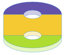
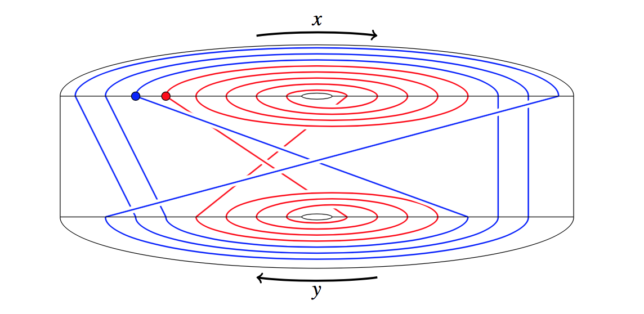
Start with a 4-dimensional ball to which we attach two handles (like the handle on a coffee mug). Formally these handles are called one-handles. So we have now attached two one-handles. We then label each handle so we can keep track of which is which. Let us call the purple one [latex]x[/latex] and the green one [latex]y[/latex]. Notice the image is a 3-dimensional depiction of our 4-manifold.We then want to glue two 4-balls onto this manifold to close up the two holes that we introduced when we attached the two one-handles in the beginning. But we will glue them on in a non-trivial way. We will follow along the two paths (red and blue) shown above. If you start from the blue dot and walk along, you’ll find the blue path goes along the [latex]x[/latex]-handle, then [latex]y[/latex], then [latex]x[/latex], then the [latex]y[/latex]-handle backwards, then [latex]x[/latex] backwards, then [latex]y[/latex] backwards, and return to the blue dot. We describe this blue path as [latex]xyxy^{-1}x^{-1}y^{-1}[/latex] and the red one is [latex]x^5y^{-4}[/latex].
We started with a 4-ball, introduced two holes, then closed off those holes. So we’re back to having just a ball. Make a copy of that ball. Then match up the boundaries of the two balls. And voila: we get a 4-dimensional sphere.
This sphere we constructed is described by the finitely presented group [latex]G = \langle x,y \mid xyx=yxy. x^5 = y^4 \rangle[/latex], which you can read all about in the beginning of Kirby’s Topology of 4-manifolds.
That’s essentially the entire construction.
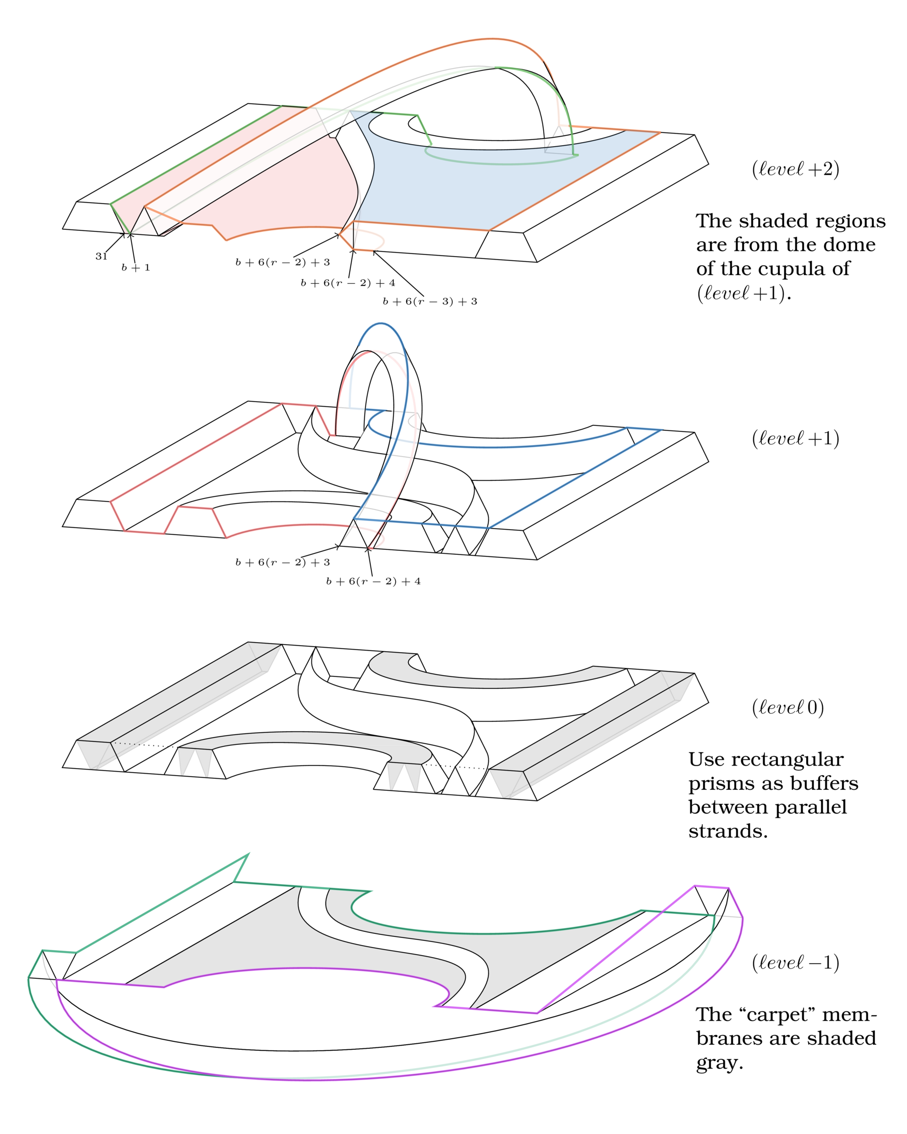
We developed a few simplicial versions of this procedure. It was a bit involved (enough for me to get a PhD), but we produced some nice pictures. Here’s a taste. For more details, check out the dissertation or the preprint.
We know that the manifolds we constructed are proper 4-spheres by Akbulut’s proof and the fact that in dimension 4, PL=DIFF. Yet, none of the sphere recognition heuristic software we know of have been able to correctly recognize them to be spheres. To our knowledge, these are the only such examples.
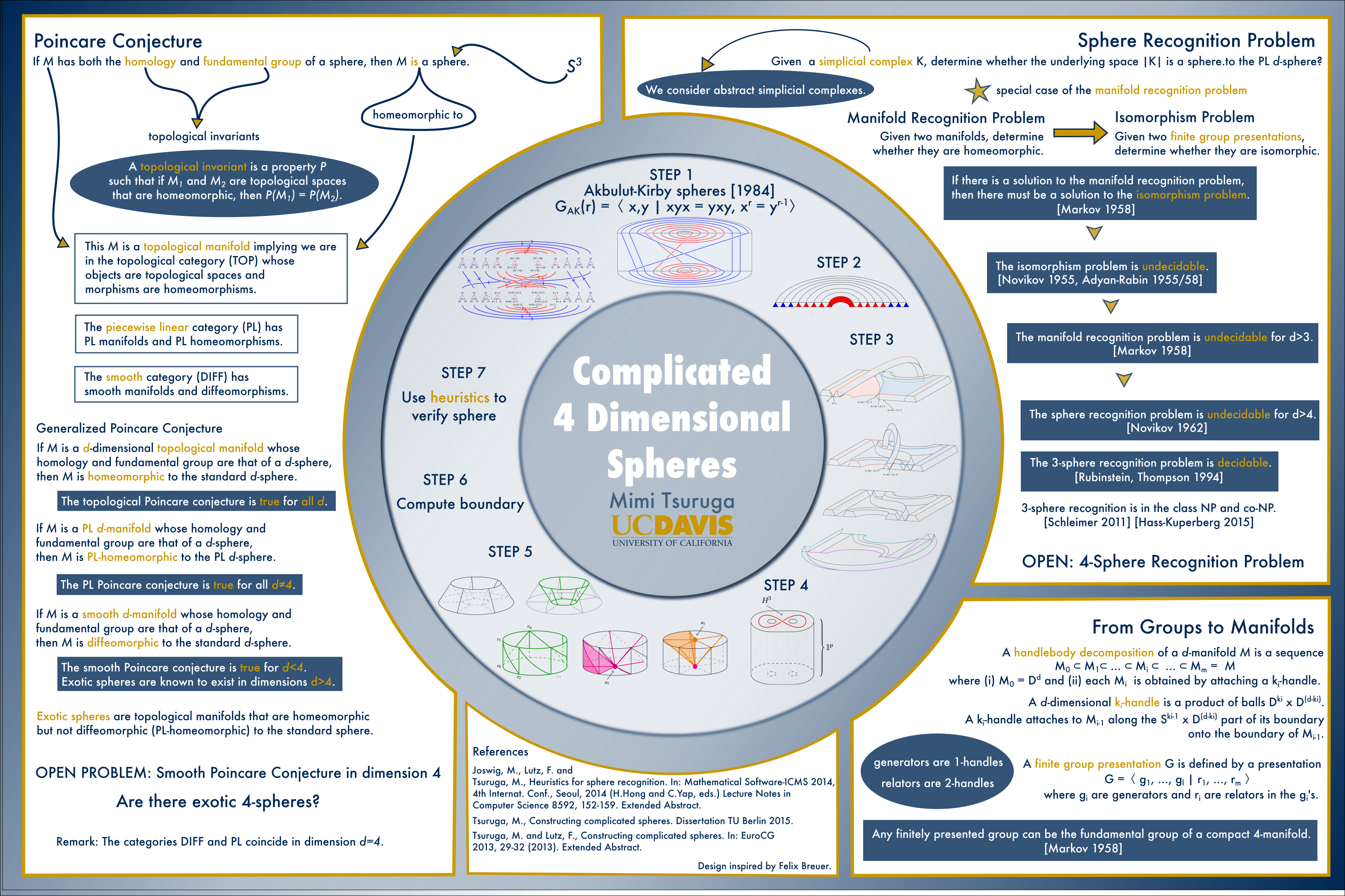
For a more graphical summary of this project, check out this poster that was presented at the MSRI Modern Math Workshop at SACNAS 2015.
J Hass and G Kuperberg. The complexity of recognizing the 3-sphere. Oberwolfach Reports, 24:1425–1426, 2012.
A Markov. The insolubility of the problem of homeomorphy. Dokl. Akad. Nauk SSSR, 121:218–220, 1958.
JH Rubinstein. An algorithm to recognize the 3-sphere. In S. D. Chatterji, editor, Proc. Internat. Congr. of Mathematicians, ICM ’94, Zürich, Volume 1, pages 601–611, Basel, 1995. Birkhäuser Verlag.
S Schleimer. Sphere recognition lies in NP. In Low-dimensional and symplectic topology, volume 82 of Proc. Sympos. Pure Math., pages 183– 213. Amer. Math. Soc., Providence, RI, 2011.
After a few hours of frustrated head bashing against my desk, I’ve finally figured out a way to add a directory containing a custom class file to my TeX search path. So before I forget the vital — yet simple — two steps, I will record them here. (Yep, that’s 4 whole hours for 2 lines of code.)
Let’s assume you’ve created an amazingly useful class file that is useful to no one else but you. (This would also apply for a custom style file (.sty) as well.) And say you want to use that class for more than one LaTeX project. It would be easy to just have the .cls file in the same folder as your LaTeX project. But you want to have just the one .cls for multiple LaTeX projects.
For this example, I’m going to call that file syllabus.cls. Let’s put that into its own unusually named folder ~/some/path/syllabus/syllabus.cls
Before we move ahead to the two lines of code, you’ll need to learn a bit about your LaTeX installation. This is the head-bashing part.
(In case you’re curious: I’m on a Mac OSX (Yosemite) with TeX-Live 2015. Also, I use TeX-lipse (with Skim) for my editor.)
Open your Terminal and type
kpsewhich --var-value TEXMFLOCAL
For me, this returns /usr/local/texlive/texmf-local
From the many posts I read on tex.stackexchange, I expected that it would be enough to place my syllabus folder right here. But it turns out life is not so kind.
One needs to dig a bit deeper to: /usr/local/texlive/texmf-local/tex/latex/local
I don’t know if this is true for everybody, but that was the case for me.
I’ve had a rather long blog-hiatus these last few months despite having just started it. It turns out that the last year of a PhD program — attending conferences, submitting articles, applying for jobs, oh, and writing that pesky dissertation — with a toddler in tow is rather challenging (who knew?) and maintaining a blog somehow ended up taking a backseat, way waay in the back. But, actually, I did write several posts. I just never published them.
These posts sat in my drafts folder collecting dust because they were rants. Rants about academia. They detailed my frustration and disappointment with this world that I had idealized as an undergraduate student. Before my life as a grad student, you would have been able to see twinkling stars reflected in my eyes as I gazed up at Professor so-and-so and their superstar academic life.
A few weeks ago, as I started preparing my applications for postdoc positions, I deleted all of those posts. For the same reason that I never published them in the first place. For fear of political repercussions. I didn’t want to lose a chance to get some job because of some opinion I happen to have. And besides, they were just rants, right?
This morning, I read this letter from a guy who was so frustrated with academia that he quit just a few months before he finished. It echoed some of the frustration I felt a few months ago and reignited the anger I attempted to bury back then. Putting aside the comments about his possible burnout, I think the points he makes are valid.
Right off the bat, let me be very clear that I love the research I’m doing and the people I work with now. I really, really do.
But I have definitely seen the awful things mentioned in that letter. And it’s forced me to reevaluate my possible career direction, especially now that I’m getting ready to send out my applications for whatever may come next.
All that political mumbo-jumbo that academia claims to exist above, it’s all there lurking behind the closed meetings attended by greedy, ambitious tenured faculty and cautious, conservative administrators. At least in industry, all that cut-throat deception and lord-of-the-flies competition for prestige is out in the open, even expected. No one pretends to be “better than those money-grubbing capitalists”. If I can’t escape dealing with assholes, better the devil you know — or at least the devil that doesn’t hide his horns.
But there are also great people in academia. Who want to change academia from the inside. Who believe that other people in academia also want the academy to be great. These are the people who got me interested in academia in the first place.
The problem for me now is not that I think academia is devoid of good people. And it’s certainly not that I’ve stopped believing in its message. I do. I still want to be part of the group who endeavors to extend human knowledge and to openly and freely share that understanding.
The biggest problem I have is that I get it. I mean, I need to eat, too. And the work I just spent six months of my life on “for the betterment of society” should at least feed me and my family for the next six months of painstaking work, right?
But I believe the system isn’t broken. It’s just been around so long that people have started exploiting some of its loop-holes. The system just needs to evolve. Install some anti-virus software and update it from time-to-time.
I remember I once had a conversation with Peter some years ago — way before I ever got a behind-the-scenes look at an academic Board meeting — about how the people who are able to talk about change (the tenured bunch) are too comfortable to ruffle any feathers and the people who have ideas to bring about change (the postdocs and tenure-tracked lot) are too scared to say anything publicly.
So I have an idea.
The anti-virus protection for academia has to begin with a discussion. We have to identify its flaws and consider the possible ways of correcting them. But most people who can say anything worth hearing can’t because they may lose their jobs or grants or whatever.
Now a blog seems to me to be a great place to begin and have a discussion. And it may even be possible to have this discussion anonymously — as long as it is thoroughly monitored and identities are well masked.
I will gladly take on the role of monitor and editor for such a blog. I’ll even offer up my blog space for this (with Peter’s permission, of course, since this is his server space). If enough people get involved, we could perhaps have a great thing going.
Anyone who wants to be part of this conversation should email me personally. After I’ve vetted the authors to my satisfaction, I would then collect relevant topics, edit their content to remove any identifiable markers and post them on this or some new blog. Any comments for the posts will go through a similar process.
Visitors to the blog will feel like they are listening in on a conversation I am having with myself. The “voice” of the blog will always be mine though the thoughts behind it may be that of many.
In my last post, we talked about homology and Betti numbers. We had a very simple example with a simplicial complex $K$ and we were able to easily compute $H_1(K)$ and $\beta_1(K)$. But that wasn’t really the whole story.
To write an algorithm that can find the Betti numbers of any given (finite) simplicial complex, we actually need to know more about how to read off the geometric information of the input complex and what to do with that information.
(Most of the material in this post can be found in Munkres, Elements of Algebraic Topology $\S 11$.)
Let’s first lay out the basics.
A(n abstract) simplicial complex is a collection $K$ of finite non-empty sets such that if $\sigma$ is an element of $K$, so is every non-empty subset of $\sigma$.
An element $\sigma$ of $K$ is called a simplex of $K$; its dimension is one less than the number of its elements. We may refer to $\sigma$ as a $p$-simplex or denote it as $\sigma^p$ to indicate its dimension $p$.
Each nonempty subset $\tau$ of $\sigma$ is called a face of $\sigma$; we say that $\tau$ is incident to $\sigma$ and denote it $\tau \prec \sigma$.
The dimension $d$ of $K$ is the largest dimension of one of its simplices. A $d$-simplex of $K^d$ is called a facet of $K$.
Given a finite complex $L$, we say that there is a labeling of the vertices of $L$, which means that there is a surjective function $f$ mapping the vertex set of $L$ to a set of labels (usually $\{0,1,2, \dots\}$ or $\{1,2, \dots\}$). Corresponding to this labeling is an abstract complex $K$ whose vertices are the labels and whose simplices consist of all sets of the form $\{f(v-0), f(v_1), \dots, f(v_n)\}$, where $v_0, \dots, v_n$ span a simplex of $L$.
This labeling mumbo-jumbo is essentially formalizing the obvious. We want to refer to specific simplices of $K$ and the convention used is to name it by its vertices.
One important property of a simplicial complex is that for every cell $\sigma$ in $K$, all of the faces of $\sigma$ are also in $K$. This property we will exploit when setting up our problem.
Step 1: Setting up the input
For a given simplicial complex $K^d$ of dimension $d$, we need only the set of $d$-simplices of $K$, the facets of $K$, as the input for our algorithm. With this list we can determine all the simplices of $K$ and their connectivity.
We’re now ready to set up all of our $C_p$’s, the $p$-chain groups of $K$. Actually, what we really have is the just the basis elements of the $C_p$, but that’s all we need. For each $p= 0, \dots, d$, the basis of $C_p$ is the set of $p$-simplices of $K$.
Let $F$ be our facet list of $K^d$. Every element of $F$ contains $(d+1)$ elements. For any $i=0, \dots, d$, the basis of $C_i$ will be the union of all subsets of elements of $F$ of length $i+1$.
So if $K$ is just two triangles, $F = \{ [1 \, 2\, 3],[2\, 3\, 4]\}$, then the basis of $C_1(K)$ is just the set of edges of $K$ or $\{[1\, 2], [1\, 3], [2\, 3], [2\, 4], [3\, 4]\}$, all length 2 subsets of elements of $F$. Even though edge $[2\, 3]$ is in both triangles, we only need to count it once.
Step 2: Setting up the boundary map
The boundary maps $\partial_p$ are the main characters in homology groups. From group theory, we know that all we really need to know about a homomorphism $f: G \to G’$ is how $f$ acts on the basis elements of $G$ in terms of the basis elements of $G’$.
More formally, let’s take a look at this definition:
Definition (matrix of a homomorphism) Let $G$ and $G’$ be free abelian groups with bases $a_1, \dots, a_n$ and $a_1′, \dots, a_m’$, respectively. If $f: G \to G’$ is a homomorphism, then $$f(a_j) = \sum_{i=1}^{m} \lambda_{ij}a_i’$$ for unique integers $\lambda_{ij}$. The matrix $(\lambda_{ij})$ is called the matrix of $f$ relative to the given bases for $G$ and $G’$.
The chain groups $C_p$ are the free abelian groups. And our boundary maps $\partial_p: C_p \to C_{p-1}$ are the homomorphisms between them. To learn more about the boundary maps, we must further analyze the matrix of $\partial_p$.
Step 3: Computing the Smith Normal Form
To understand what the boundary map is doing, let’s first recall a nice theorem from algebra.
Theorem (normal form) Let $G$ and $G’$ be free abelian groups of ranks $n$ and $m$, respectively; let $f: G \to G’$ be a homomorphism. Then there are bases for $G$ and $G’$ such that, relative to these bases, the matrix of $f$ has the form $$B=\left[\begin{array}{c|c}\begin{matrix}b_1 & ~ & 0 \\ ~ & \ddots & ~ \\ 0 & ~&b_q\end{matrix} & 0 \\ \hline 0 & 0\end{array}\right]$$ where $b_i \ge 1$ and $b_1 | b_2| \dots | b_q$.
This matrix is uniquely determined by $f$ and is called the normal form for the matrix of $f$.
To get from some jumbled up matrix $(\lambda_{ij})$ to its normal form, we perform what are called elementary row and column operations. These operations are
exchange row $i$ and row $k$
multiply row $i$ by $-1$
replace row $i$ by (row $i$) + $q$ (row $k$), where $q$ is an integer and $k \ne i$,
plus the 3 respective column operations.
Perhaps you remember seeing the elementary row operations from linear algebra. It’s important to note that here we’re only allowing integer multiplication for operation type 3 (and 6 for the column operations).
Step 4: What it means
Recall what our goal was: to compute the homology groups of some finite simplicial complex $K$. And we know that all homology groups $H_p \cong \mathbb{Z}_{t_1} \times \cdots \times \mathbb{Z}_{t_k} \times \mathbb{Z}^{\beta}$ can be written in terms of their Betti numbers $\beta$ and their torsion coefficients $t_1, \dots t_k$.
Now that we have the normal form for all the boundary maps $\partial_p$ for $p=0, \dots, d$, we can easily read off this information.
Torsion coefficients: The entries of the normal form for the matrix of $\partial_p: C_p \to C_{p-1}$ that are greater than 1 are the torsion coefficients of $K$ in dimension $p-1$.
Betti numbers: Let $B_i$ be the normal form for the matrix of $\partial_i: C_i \to C_{i-1}$. The Betti number of $K$ in dimension $p$ is $$\beta_p = \text{rank} C_p – \text{rank} B_p – \text{rank} B_{p+1}.$$
So we’re done.
Or we should be, but we’re not. If we’re done why, then, are people still working on developing homology algorithms?


 We then want to glue two 4-balls onto this manifold to close up the two holes that we introduced when we attached the two one-handles in the beginning. But we will glue them on in a non-trivial way. We will follow along the two paths (red and blue) shown above. If you start from the blue dot and walk along, you’ll find the blue path goes along the [latex]x[/latex]-handle, then [latex]y[/latex], then [latex]x[/latex], then the [latex]y[/latex]-handle backwards, then [latex]x[/latex] backwards, then [latex]y[/latex] backwards, and return to the blue dot. We describe this blue path as [latex]xyxy^{-1}x^{-1}y^{-1}[/latex] and the red one is [latex]x^5y^{-4}[/latex].